Section 5 Structuring
Data structuring is the process of correcting, rearranging, or removing inaccurate records from raw data so that, after the treatment, the transformed data will be easy to analyze. The variable names, types, and values must be consistent and uniform. The focus here is on the appearance of the data. We often restructure data so that we can merge two dataframes with pairable attributes, combine several sources describing the same event, or prepare data for intense statistical analysis that requires consistent and complete data. Whatever the purpose, having clean data is a good habit regardless of application or functionality. If somebody else picks up your project, you do not want to have to explain to them the complications and intricacies of messy data. The first stage of structuring is to make sure that your read-in process gave you data of the type that you anticipated or intended. Before we can do that, we should learn how to access specific parts of the data for examination.
5.1 Accessing Data in R
Once you have read in your data, you may want to look, change, or perform calculations on a specific part or element. Keep in mind that R uses 1-indexing instead of 0-indexing, which other languages like Python employ. 1-indexing means that you start counting from the number 1 instead of 0. To access a range of values in a dataframe, you can specify a set of numbers or column names. Let’s create a dataframe below so that you can get a sense of how this works.
x <- data.frame(replicate(5, sample(1:10,20,rep=TRUE)))
names(x) <- c("One", "Two", "Three", "Four", "Five")
What we’ve just done above is create a dataframe with 5 columns, each of which has 20 rows populated by a random number between 1 and 10. The names of these columns are One, Two, Three, Four, and Five respectively. Let’s say that we want to access just the first three rows of the third and fourth columns. We can do that one of two ways:
The first line shows how we use indexing to access data. The rows are listed first, then after a comma the columns are listed. If we want a range of values, we use ‘:’ to indicate we want every number between the two values. 1:4 means we want rows 1, 2, 3, and 4 while just typing 4 means we want just row 4. We use the same logic for columns. However, if we want to access columns by name, we can generate a vector within c(), which is the R shorthand way of writing a vector. Each value within c() is treated as a single variable, separated by commas. In the example, we typed c("Three", "Four") to get the third and fourth columns. Whatever the names of the columns that you want are, you can use this method to access them. You can also use c() to get a non-consecutive set of numbers. Say we want the first, third, and fifth column. We could use c(1,3,5) to get just these columns.
Let’s say we just want one column from a dataframe to use for examination or manipulation. We can use the $ character to clarify which one we want by name. You will see this all over R scripts, as it is very common to want to access a particular column or item in a list in its entirety.
The first command gives us just the fifth column of the frame. The second command gives us the sixth to eighth row of the fifth column, using the same square bracket [] indexing as before. Typically, square brackets are reserved for indexing, and parentheses are used for functions.
One final method of subsetting is throuch exclusion. You can type - in front of a number if you want to access everything but a single column. For example, instead of typing c(1,2,3,5) to get all columns except for the fourth, we can write -4.
5.2 Data types
One type of anomaly that we may encounter is the coercion of irrelevant data types to variables. This is very common for numerically coded variables, or variables that have distinct levels. First we read in our data by the method we practiced in the earlier chapter:
If we read in the same SPSS data from the Reading data section, we get the coded values instead of the labels.
## # A tibble: 6 x 9
##   Zone     Q4           Q5    Q6           Q7     Q10   Q50     Q51          Q59
##   <chr> <dbl>    <dbl+lbl> <dbl>    <dbl+lbl> <dbl+l> <dbl> <dbl+l>    <dbl+lbl>
## 1 A         2 3                0 3 [Moderate…  2 [No]  1928 1 [Mal…  4 [$70,000…
## 2 A         1 4                0 3 [Moderate…  2 [No]  1962 1 [Mal… NA
## 3 A         3 4                0 3 [Moderate…  2 [No]  1931 2 [Fem…  6 [Over $2…
## 4 A         3 6                1 1 [Fully Pr…  2 [No]  1950 1 [Mal…  5 [$100,00…
## 5 A         2 1 [Not Worr…     0 2 [Very Pre…  2 [No]  1948 1 [Mal…  5 [$100,00…
## 6 A         5 4                0 2 [Very Pre…  2 [No]  1938 2 [Fem… NA
It appears as though some of the categorical data was read in as integers. This is a quirk of R, that if left unchanged can drastically change the outcome of your analyses. To access the specific type of data of one column, we can use the class() function, then pass the name of the frame and column we are trying to access using the technique outlined above:
## [1] "numeric"Q6 is meant to be categorical, not numeric. If we run summary(data), we get this unintended result which affects several columns:
## Warning in mask$eval_all_mutate(dots[[i]]): NAs introduced by coercion## Zone Q4 Q5 Q6
## Min. : NA Min. : 0.000 Min. :1.000 Min. :0.0000
## 1st Qu.: NA 1st Qu.: 2.000 1st Qu.:1.000 1st Qu.:0.0000
## Median : NA Median : 2.000 Median :2.000 Median :0.0000
## Mean :NaN Mean : 2.537 Mean :1.617 Mean :0.4191
## 3rd Qu.: NA 3rd Qu.: 3.000 3rd Qu.:2.000 3rd Qu.:1.0000
## Max. : NA Max. :20.000 Max. :2.000 Max. :4.0000
## NA's :1130 NA's :134 NA's :968 NA's :116
## Q7 Q10 Q50 Q51 Q59
## Min. :1.000 Min. :1.000 Min. : 19 Min. :1.00 Min. :1.000
## 1st Qu.:2.000 1st Qu.:2.000 1st Qu.:1944 1st Qu.:1.00 1st Qu.:3.000
## Median :3.000 Median :2.000 Median :1955 Median :2.00 Median :4.000
## Mean :2.674 Mean :1.796 Mean :1944 Mean :1.55 Mean :3.715
## 3rd Qu.:3.000 3rd Qu.:2.000 3rd Qu.:1966 3rd Qu.:2.00 3rd Qu.:5.000
## Max. :5.000 Max. :2.000 Max. :1992 Max. :2.00 Max. :6.000
## NA's :114 NA's :123 NA's :47 NA's :38 NA's :112Q4 and Q50 are the only variables that are supposed to be numeric, but here everything is treated as numeric, even when it was originally categorical data, which is incorrect. We might also want to treat Zone as a factor so that we can examine groups collectively based on this metric.
We can easily convert data types into factors using either dplyr::mutate_at() and applying as.factor function to the variables. Examples of both are given below:
# Converting data types
updated_data <- data %>% mutate_at(vars(-Q4, -Q6, -Q50), as_factor)

# Alternately, for specific columns
data$Q6 <- as.factor(data$Q6)
And now we can get the full summary statistics in the form that we want:
##  Zone          Q4               Q5            Q6
##  A:684   Min.   : 0.000   5      :244   Min.   :0.0000
##  B:446   1st Qu.: 2.000   4      :211   1st Qu.:0.0000
##          Median : 2.000   3      :169   Median :0.0000
##          Mean   : 2.537   6      :129   Mean   :0.4191
##          3rd Qu.: 3.000   2      :104   3rd Qu.:1.0000
##          Max.   :20.000   (Other):162   Max.   :4.0000
##          NA's   :134      NA's   :111   NA's   :116
##                    Q7        Q10           Q50           Q51
##  Fully Prepared     : 93   Yes :205   Min.   :  19   Male  :491
##  Very Prepared      :326   No  :802   1st Qu.:1944   Female:601
##  Moderately Prepared:438   NA's:123   Median :1955   NA's  : 38
##  A Little Prepared  :137              Mean   :1944
##  Not at all Prepared: 22              3rd Qu.:1966
##  NA's               :114              Max.   :1992
##                                       NA's   :47
##                 Q59
##  Less than $15,000: 81
##  $15,000-$39,999  :169
##  $40,000-$69,999  :215
##  $70,000-$99,999  :190
##  $100,000-$199,999:220
##  Over $200,000    :143
##  NA's             :112
As we can see from the summary, there might still be anomalies with the variables:
Q4: Number of storms experienced: The mean value is 2.5 but the max value is 20, which suggests heavily right skewed data.Q50: Birth year: Some respondent answered 19 which is incorrect. It’s pretty clearly a typo, because nobody is 2,001 years old. We may also consider transforming this column into age instead of birth year, which makes it easier to interpret.
Perpetually in data analysis, the issue of missing values and how to deal with them comes up. We can see here that this dataset is no different, with several NA values across the board. We will talk at length about missing data later on in the next chapter on Data Cleaning.
5.3 Inspecting the data
In order to structure a dataset, we need to not only detect the anomalies within the data, but also decide what to do with them. Such anomalies can include values that are stored in the wrong format (ex: a number stored as a string), values that fall outside of the expected range (ex: outliers), values with inconsistent patterns (ex: dates stored as mm/dd/year vs dd/mm/year), trailing spaces in strings (ex: data vs data), or other logistical issues.
With our data successfully read in above, we can examine both structure and summary statistics for numerical and categorical variables.
## tibble [1,130 × 3] (S3: tbl_df/tbl/data.frame)
##  $ Zone: chr [1:1130] "A" "A" "A" "A" ...
##   ..- attr(*, "format.spss")= chr "A9"
##   ..- attr(*, "display_width")= int 1
##  $ Q4  : num [1:1130] 2 1 3 3 2 5 3 5 1 2 ...
##   ..- attr(*, "label")= chr "Q4. Since the beginning of 2009, how many hurricanes and tropical storms, if any, hit your city or town on or n"| __truncated__
##   ..- attr(*, "format.spss")= chr "F2.0"
##   ..- attr(*, "display_width")= int 2
##  $ Q5  : dbl+lbl [1:1130]  3,  4,  4,  6,  1,  4,  6,  4,  3,  6,  7,  5,  7,  ...
##    ..@ label      : chr "Q5. Generally speaking, when a hurricane or tropical storm is approaching your city or town, how worried do you"| __truncated__
##    ..@ format.spss: chr "F1.0"
##    ..@ labels     : Named num [1:2] 1 7
## .. ..- attr(*, "names")= chr [1:2] "Not Worried At All" "Extremely Worried"## Min. 1st Qu. Median Mean 3rd Qu. Max. NA's
## 0.000 2.000 2.000 2.537 3.000 20.000 134## Fully Prepared Very Prepared Moderately Prepared A Little Prepared
## 93 326 438 137
## Not at all Prepared NA's
## 22 114Here we will look at the output of a few other key functions. Calling head() will by default show you the first six rows of a dataframe. If you want to see more or fewer rows, simply put a comma in after the dataframe’s name and write the number of rows you want to display. Calling tail() will give you the exact opposite, displaying the last n rows of data, with the default again set to six.
## # A tibble: 10 x 9
##    Zone     Q4           Q5 Q6              Q7     Q10   Q50     Q51         Q59
##    <chr> <dbl>    <dbl+lbl> <fct>    <dbl+lbl> <dbl+l> <dbl> <dbl+l>   <dbl+lbl>
##  1 A         2 3            0     3 [Moderate…  2 [No]  1928 1 [Mal…  4 [$70,00…
##  2 A         1 4            0     3 [Moderate…  2 [No]  1962 1 [Mal… NA
##  3 A         3 4            0     3 [Moderate…  2 [No]  1931 2 [Fem…  6 [Over $…
##  4 A         3 6            1     1 [Fully Pr…  2 [No]  1950 1 [Mal…  5 [$100,0…
##  5 A         2 1 [Not Worr… 0     2 [Very Pre…  2 [No]  1948 1 [Mal…  5 [$100,0…
##  6 A         5 4            0     2 [Very Pre…  2 [No]  1938 2 [Fem… NA
##  7 A         3 6            1     3 [Moderate…  2 [No]  1977 2 [Fem… NA
##  8 A         5 4            0     3 [Moderate…  2 [No]  1964 2 [Fem… NA
##  9 A         1 3            0     3 [Moderate…  2 [No]  1976 1 [Mal…  3 [$40,00…
## 10 A 2 6 0 2 [Very Pre… 2 [No] 1964 2 [Fem… 6 [Over $…## # A tibble: 10 x 9
## Zone Q4 Q5 Q6 Q7 Q10 Q50 Q51 Q59
## <chr> <dbl> <dbl+l> <fct> <dbl+lbl> <dbl+lb> <dbl> <dbl+lb> <dbl+lbl>
## 1 B 1 2 0 4 [A Little P… 2 [No] 1980 1 [Male] 3 [$40,000-…
## 2 B 2 2 0 3 [Moderately… 2 [No] 1977 2 [Fema… 4 [$70,000-…
## 3 B 4 4 1 2 [Very Prepa… 1 [Yes] 1962 2 [Fema… 2 [$15,000-…
## 4 B 2 5 0 1 [Fully Prep… 2 [No] 1946 1 [Male] 5 [$100,000…
## 5 B NA 4 <NA> 1 [Fully Prep… 1 [Yes] 1957 2 [Fema… 1 [Less tha…
## 6 B 1 4 1 4 [A Little P… 1 [Yes] 1987 2 [Fema… 6 [Over $20…
## 7 B 2 5 0 3 [Moderately… 2 [No] 1953 1 [Male] 4 [$70,000-…
## 8 B NA 4 4 2 [Very Prepa… 2 [No] 1973 2 [Fema… 1 [Less tha…
## 9 B 2 5 0 3 [Moderately… 2 [No] 1980 1 [Male] 5 [$100,000…
## 10 B 2 2 0 4 [A Little P… 2 [No] NA 2 [Fema… 3 [$40,000-…To find the number of rows and columns your dataframe has, call dim(). To find just the rows, use nrow(). To find just the columns, use ncol(). Calling either names() or colnames() will give you the names of the columns. If your data has row names (which is not always the case), you can use rownames() to access those.
## [1] 1130 9## [1] 1130## [1] 9## [1] "Zone" "Q4" "Q5" "Q6" "Q7" "Q10" "Q50" "Q51" "Q59"We can also plot the data to visualize the distribution of variables using the dplyr and magrittr
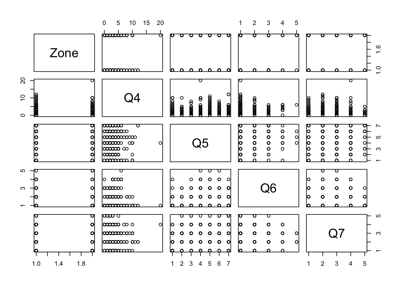
If you use these techniques and see an outlier, whether it be an abnormally large or small number, you can use either the min() or max() function to get the specific value. Because we have missing values, we need to pass the argument na.rm = TRUE to ignore all NA values when calculating these. For several numerical evaluations, R makes sure to explicitly highlight the presence of NA values, which are treated as unknowns. Because R does not know if the missing value could have been the minimum or maximum, it will tell you that this calculation is NA unless you explicitly give it permission to ignore these missing values.
## [1] 20## [1] 195.4 Subsetting and Filtering
We can remove incorrect or missing row values by using dplyr::filter:
# Removing rows where birth year is irrelevant
# Here we decided that all birth year must be greater 1900
updated_data <- data %>% filter(Q50 > 1900)

# Now if we re-run its summary we get the following
summary(updated_data$Q50)
## Min. 1st Qu. Median Mean 3rd Qu. Max.
## 1908 1945 1955 1956 1966 1992# Removing rows with birth year greater than 1900 and missing responses for Q4
updated_data <- data %>% filter(Q50 > 1900, !is.na(Q4))
summary(updated_data$Q50)## Min. 1st Qu. Median Mean 3rd Qu. Max.
## 1908 1944 1954 1955 1965 1990## Min. 1st Qu. Median Mean 3rd Qu. Max.
## 0.000 2.000 2.000 2.522 3.000 20.000We can also select for only the variables that we are interested in using the function dplyr::select:
# Creating a new dataframe with only zone, gender, and income columns
updated_data <- data %>% select(Zone, Q59, Q51)
head(updated_data, 10)
## # A tibble: 10 x 3
## Zone Q59 Q51
## <fct> <fct> <fct>
## 1 A 4 1
## 2 A <NA> 1
## 3 A 6 2
## 4 A 5 1
## 5 A 5 1
## 6 A <NA> 2
## 7 A <NA> 2
## 8 A <NA> 2
## 9 A 3 1
## 10 A 6 2
It is also possible to split the dataset into multiple dataframes by number of rows using split():
# To split the dataset into multiple dataframes of 10 rows each
max_number_of_rows_per_dataframe <- 10
total_number_rows_in_the_current_dataset <- nrow(data)
sets_of_10rows_dataframes <- split(data,
                                   rep(1:ceiling(total_number_rows_in_the_current_dataset/max_number_of_rows_per_dataframe),
                                       each=max_number_of_rows_per_dataframe,
                                       length.out=total_number_rows_in_the_current_dataset)
                                   )
# Here are the first 2 dataframes
sets_of_10rows_dataframes[[1]] # or sets_of_10rows_dataframes$`1`
## # A tibble: 10 x 9
## Zone Q4 Q5 Q6 Q7 Q10 Q50 Q51 Q59
## <fct> <dbl> <fct> <fct> <fct> <fct> <dbl> <fct> <fct>
## 1 A 2 3 0 3 2 1928 1 4
## 2 A 1 4 0 3 2 1962 1 <NA>
## 3 A 3 4 0 3 2 1931 2 6
## 4 A 3 6 1 1 2 1950 1 5
## 5 A 2 1 0 2 2 1948 1 5
## 6 A 5 4 0 2 2 1938 2 <NA>
## 7 A 3 6 1 3 2 1977 2 <NA>
## 8 A 5 4 0 3 2 1964 2 <NA>
## 9 A 1 3 0 3 2 1976 1 3
## 10 A 2 6 0 2 2 1964 2 6## # A tibble: 10 x 9
## Zone Q4 Q5 Q6 Q7 Q10 Q50 Q51 Q59
## <fct> <dbl> <fct> <fct> <fct> <fct> <dbl> <fct> <fct>
## 1 A 2 7 2 1 1 1937 2 <NA>
## 2 A 3 5 0 2 2 1943 1 4
## 3 A 2 7 0 2 2 1954 2 5
## 4 A 2 5 0 2 2 1959 2 5
## 5 A 4 1 <NA> 2 2 1936 2 6
## 6 A 1 3 1 3 1 1963 1 6
## 7 A 2 3 1 2 1 1950 2 5
## 8 A 4 6 0 3 2 NA <NA> <NA>
## 9 A 0 4 0 2 2 1941 1 5
## 10 A NA <NA> <NA> <NA> <NA> 1952 2 55.5 Changing cell values
As we mentioned earlier, it is best if Q50 is stored as an age variable instead of the default birth year. Q50 is a numeric variable and we can simply change it by using dplyr::mutate()
With the filtered data, we can replace all of the values in Q50 with 2020 - Q50 like so:
# Replacing Q50 values to their age in 2020
updated_data <- data %>% mutate(Q50 = 2020 - Q50)
head(updated_data, 10)
## # A tibble: 10 x 9
## Zone Q4 Q5 Q6 Q7 Q10 Q50 Q51 Q59
## <fct> <dbl> <fct> <fct> <fct> <fct> <dbl> <fct> <fct>
## 1 A 2 3 0 3 2 92 1 4
## 2 A 1 4 0 3 2 58 1 <NA>
## 3 A 3 4 0 3 2 89 2 6
## 4 A 3 6 1 1 2 70 1 5
## 5 A 2 1 0 2 2 72 1 5
## 6 A 5 4 0 2 2 82 2 <NA>
## 7 A 3 6 1 3 2 43 2 <NA>
## 8 A 5 4 0 3 2 56 2 <NA>
## 9 A 1 3 0 3 2 44 1 3
## 10 A 2 6 0 2 2 56 2 6# It is also possible to leave Q50 untouched and store the results into a new column
updated_data <- data %>% mutate(age = 2020 - Q50)
head(updated_data, 10)## # A tibble: 10 x 10
## Zone Q4 Q5 Q6 Q7 Q10 Q50 Q51 Q59 age
## <fct> <dbl> <fct> <fct> <fct> <fct> <dbl> <fct> <fct> <dbl>
## 1 A 2 3 0 3 2 1928 1 4 92
## 2 A 1 4 0 3 2 1962 1 <NA> 58
## 3 A 3 4 0 3 2 1931 2 6 89
## 4 A 3 6 1 1 2 1950 1 5 70
## 5 A 2 1 0 2 2 1948 1 5 72
## 6 A 5 4 0 2 2 1938 2 <NA> 82
## 7 A 3 6 1 3 2 1977 2 <NA> 43
## 8 A 5 4 0 3 2 1964 2 <NA> 56
## 9 A 1 3 0 3 2 1976 1 3 44
## 10 A 2 6 0 2 2 1964 2 6 56## Min. 1st Qu. Median Mean 3rd Qu. Max.
## 28.00 54.00 65.00 64.14 75.00 112.00For a categorical variable, we use a different function: dplyr::recode_factor() or dplyr::recode(). We will apply this to Q5 as we have noticed in the previous section that not all of its values were labelled from SPSS. Here is its summary:
##    1    2    3    4    5    6    7 NA's
##   58  101  164  197  232  123   97  104
Looking back at the questionnare, here is how it was phrased:
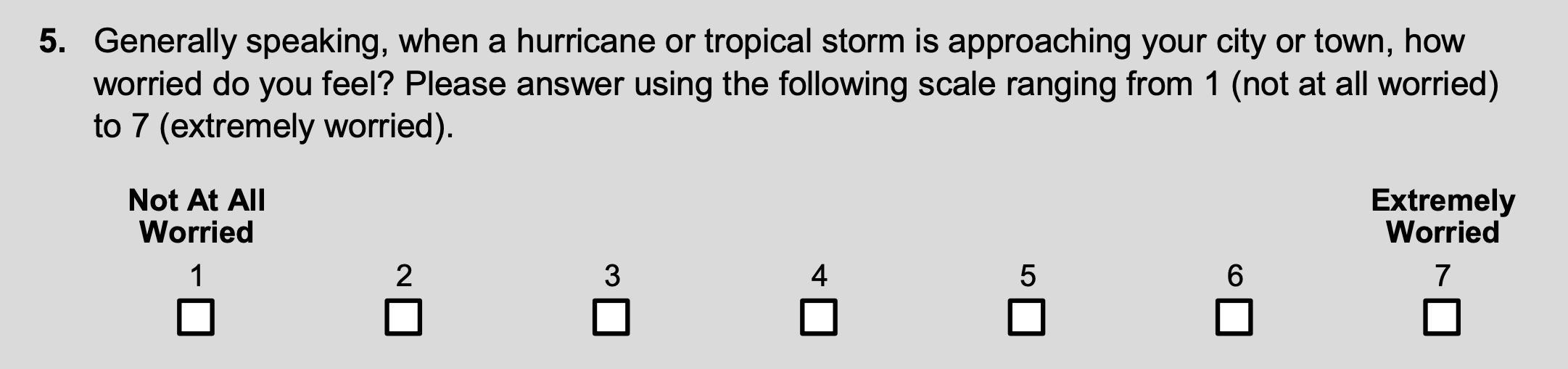
Because the survey itself does not have labels, the recoding will be up to the user. Here we chose to replace the extreme values with 1 and 7. As mentioned in the documentation: dplyr::recode() will preserve the existing order of levels while changing the values, and dplyr::recode_factor() will change the order of levels to match the order of replacements.
# Recoding Q5
recoded.with.recode <- recode(data$Q5, `Not Worried At All`="1", `Extremely Worried`="7")
summary(recoded.with.recode)
## 1 2 3 4 5 6 7 NA's
## 58 101 164 197 232 123 97 104recoded.with.recode_factor <- recode_factor(data$Q5, `Not Worried At All`="1", `Extremely Worried`="7")
summary(recoded.with.recode_factor)## 1 7 2 3 4 5 6 NA's
## 58 97 101 164 197 232 123 104We can also change cell values without external libraries like dplyr by running the following code:
# Add column age where the values are 2020 - Q50
data$age <- 2020 - data$Q50

# Replace Q5 with value "Not Worried At All" to "1"
data$Q5[data$Q5 == "Not Worried At All"] <- 1
Notice above that we used a conditional subset in the second command. Just like we used indexing earlier, we can also use a Boolean vector (True/False) to pick only rows where some condition is met. Within the [] brackets, we gave a statement: data$Q5 == "Not Worried At All" using == to indicate we want True/False for each row. This syntax will return only the entries of Q5 that are True within the condition. We then reassign the value for each of these to be 1 instead of Not Worried At All, effectively doing the same task as we did above. R is smart enough to work with vectors in this way, running the same evaluation on each entry without you specifying.
One final set of functions that can be incredibly helpful with changing cell values are gsub() and grep(). If, for instance, you want to find all entries of a column that have a specific string pattern in them, you can use grep() to locate every instance. Simply type in the pattern, and the frame over which you want the function to look. For instance, if we wanted to find every entry of a column with the word "missing" in it, we could use grep() like so:
Now let’s say that instead of simply locating every instance, we instead want to replace them with a substitute phrase. That is when we would use gsub(), which lets us substitute another phrase in. If we wanted to replace every part of every entry that says "CT" with "Connecticut", we could do so:
5.6 Pivoting the dataset
In some cases, we may want to split a column based on values, or merge multiple columns into fewer columns. A classic example is with time-stamped data. Sometimes we want rows to be days, with individual responses recorded as columns, and sometimes we want each row to be an individual, with columns representing days. It just depends on what the data are modelling. This process can be done using the tidyr package. For example, to convert the dataframe into long-format with only Zone, question, and value as columns:
# Read in the necessary package
library(tidyr)

# We have to pivot by variable type
# Pivot longer for factor variables
pivoted.longer <- data %>%
  select_if(is.factor) %>%
  pivot_longer(-Zone, names_to = "question", values_to = "value")
pivoted.longer
## # A tibble: 6,456 x 3
## Zone question value
## <fct> <chr> <fct>
## 1 A Q5 3
## 2 A Q6 0
## 3 A Q7 3
## 4 A Q10 2
## 5 A Q51 1
## 6 A Q59 4
## 7 A Q5 4
## 8 A Q6 0
## 9 A Q7 3
## 10 A Q10 2
## # … with 6,446 more rows# Then we can reshape it back to the original
pivoted.wider <- pivoted.longer %>%
group_by(question) %>% mutate(row = row_number()) %>%
pivot_wider(names_from = question, values_from = value) %>%
select(-row)
pivoted.wider## # A tibble: 1,076 x 7
## Zone Q5 Q6 Q7 Q10 Q51 Q59
## <fct> <fct> <fct> <fct> <fct> <fct> <fct>
## 1 A 3 0 3 2 1 4
## 2 A 4 0 3 2 1 <NA>
## 3 A 4 0 3 2 2 6
## 4 A 6 1 1 2 1 5
## 5 A 1 0 2 2 1 5
## 6 A 4 0 2 2 2 <NA>
## 7 A 6 1 3 2 2 <NA>
## 8 A 4 0 3 2 2 <NA>
## 9 A 3 0 3 2 1 3
## 10 A 6 0 2 2 2 6
## # … with 1,066 more rowstidyr::spread() and tidyr::gather() are the outdated equivalent of tidyr::pivot_wider() and tidyr::pivot_longer().
To merge or split columns, we can use tidyr::unite() or tidyr::separate(). For example, to merge Q7 and Q10:
# Creating a new column with responses from both Q7 and Q10
merged <- data %>% unite("Q7_Q10", Q7:Q10, sep = "__", remove = TRUE, na.rm = FALSE)
merged
## # A tibble: 1,076 x 9
## Zone Q4 Q5 Q6 Q7_Q10 Q50 Q51 Q59 age
## <fct> <dbl> <fct> <fct> <chr> <dbl> <fct> <fct> <dbl>
## 1 A 2 3 0 3__2 1928 1 4 92
## 2 A 1 4 0 3__2 1962 1 <NA> 58
## 3 A 3 4 0 3__2 1931 2 6 89
## 4 A 3 6 1 1__2 1950 1 5 70
## 5 A 2 1 0 2__2 1948 1 5 72
## 6 A 5 4 0 2__2 1938 2 <NA> 82
## 7 A 3 6 1 3__2 1977 2 <NA> 43
## 8 A 5 4 0 3__2 1964 2 <NA> 56
## 9 A 1 3 0 3__2 1976 1 3 44
## 10 A 2 6 0 2__2 1964 2 6 56
## # … with 1,066 more rows## # A tibble: 1,076 x 10
## Zone Q4 Q5 Q6 Q7 Q10 Q50 Q51 Q59 age
## <fct> <dbl> <fct> <fct> <chr> <chr> <dbl> <fct> <fct> <dbl>
## 1 A 2 3 0 3 2 1928 1 4 92
## 2 A 1 4 0 3 2 1962 1 <NA> 58
## 3 A 3 4 0 3 2 1931 2 6 89
## 4 A 3 6 1 1 2 1950 1 5 70
## 5 A 2 1 0 2 2 1948 1 5 72
## 6 A 5 4 0 2 2 1938 2 <NA> 82
## 7 A 3 6 1 3 2 1977 2 <NA> 43
## 8 A 5 4 0 3 2 1964 2 <NA> 56
## 9 A 1 3 0 3 2 1976 1 3 44
## 10 A 2 6 0 2 2 1964 2 6 56
## # … with 1,066 more rows5.7 Merging Two Dataframes
If we want to combine two dataframes based on a shared column, we can do that with a merge call. Let’s say we have two separate dataframes that discuss the same individuals. Each participant was given an ID that was recorded over the two frames, and we want one dataframe with their responses joined.
# Here we will create the simulated data described above
survey1 <- cbind(1:10, data.frame(replicate(10,sample(0:1,1000,rep=TRUE))))
survey2 <- cbind(1:10, data.frame(replicate(10,sample(0:1,1000,rep=TRUE))))

# Name the columns of both frames
names(survey1) <- c("ID", paste0("Q", 1:10))
names(survey2) <- c("ID", paste0("Q", 11:20))
The first column of each dataframe represents the participant’s ID, and the next 10 columns represent their responses to questions. We can use a merge to execute this:
With the merge command, we can do one of four types: an inner join, a left join, a right join, or a full join. With an inner join, we only include data that have an identification match in both sets. A left join saves all information from the left dataset and puts NA values in if there is not a corresponding row in the right, a right join does the opposite, preserving all of the right frame’s data, and a full join saves all rows from both of the original datasets.
The frame surveytotal now has all questions stored in the same place. If the ID column does not match up in format, this can give you issues, so make sure you only merge once your data is fully cleaned, which we will talk about in the next chapter.
We can also do two simpler combines, known as cbind() or rbind(), if the data do not need to be merged on an ID entry. Say, for example, we had two sheets of an Excel file which were completed on different days and had the exact same set of columns> If we want them to be in the same frame, one after the other, we could use an rbind() call to bind the rows like so:
# Generate the top dataframe
top <- data.frame(replicate(10, sample(0:1,1000,rep=TRUE)))
names(top) <- paste0("Row_", 1:10)

# Generate the bottom dataframe
bottom <- data.frame(replicate(10, sample(0:1,1000,rep=TRUE)))
names(bottom) <- paste0("Row_", 1:10)

# Use rbind() to bring them together
combined <- rbind(top, bottom)
If there are two frames that have the same number of rows that describe in sequence the same observations, we can use a cbind() call to combine them:
# Create the left data
left <- data.frame(replicate(10, sample(0:1,1000,rep=TRUE)))
names(left) <- paste0("Row_", 1:10)

# Create the right data
right <- data.frame(replicate(10, sample(0:1,1000,rep=TRUE)))
names(right) <- paste0("Row_", 11:20)

# Use cbind() to stick them together
combined <- cbind(left, right)
Keep in mind that this is only a valid merge if the two frames are composed of rows that represent the same observations.